Return to Main Page

Lab 10

Objective

In lab 10 we were tasked with implementing grid localization using Bayes filter.

Implementation

compute_control

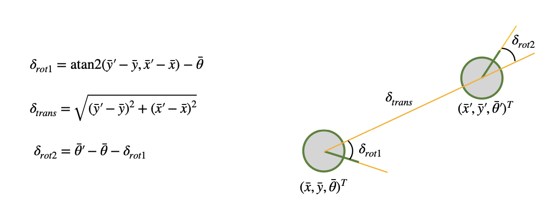
The compute_control function calculates the control parameters for the odometry motion model based on the current and previous poses. It is implemented using the equations provided in the lecture slides.

def compute_control(cur_pose, prev_pose):
    """ Given the current and previous odometry poses, this function extracts
    the control information based on the odometry motion model.

    Args:
        cur_pose  ([Pose]): Current Pose
        prev_pose ([Pose]): Previous Pose 

    Returns:
        [delta_rot_1]: Rotation 1  (degrees)
        [delta_trans]: Translation (meters)
        [delta_rot_2]: Rotation 2  (degrees)
    """
    delta_rot_1 = mapper.normalize_angle(np.degrees(np.arctan2(cur_pose[0] - prev_pose[0], cur_pose[1] - prev_pose[1])) - prev_pose[2])
    delta_trans = np.hypot(cur_pose[0] - prev_pose[0], cur_pose[1] - prev_pose[1])
    delta_rot_2 = mapper.normalize_angle(cur_pose[2] - prev_pose[2] - delta_rot_1)

    return delta_rot_1, delta_trans, delta_rot_2

odom_motion_model

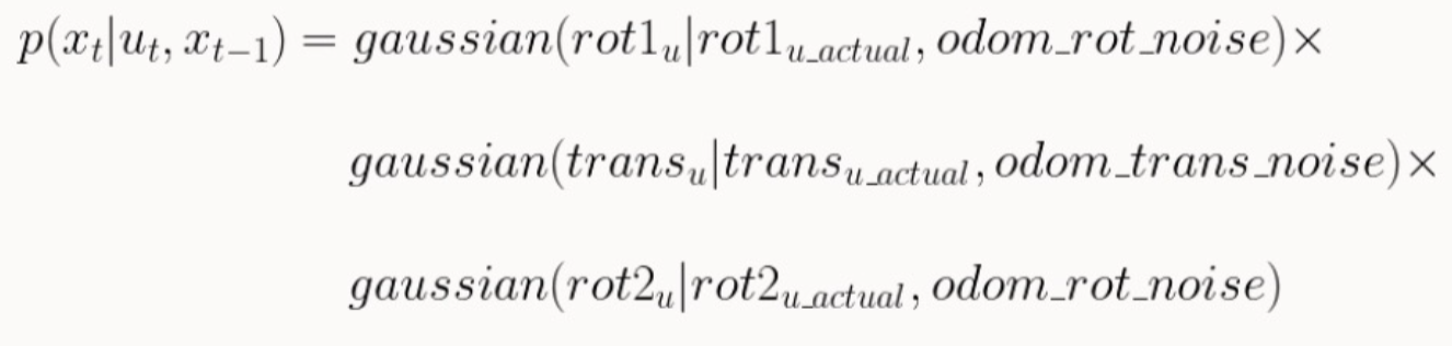
The odom_motion_model function evaluates how likely it is that the robot transitioned from prev_pose to cur_pose, given a proposed control action u. It does this by comparing the actual motion observed computed from the poses using compute_control with the expected control input u, using Gaussian probability distributions.

def odom_motion_model(cur_pose, prev_pose, u):
    """ Odometry Motion Model

    Args:
        cur_pose  ([Pose]): Current Pose
        prev_pose ([Pose]): Previous Pose
        (rot1, trans, rot2) (float, float, float): A tuple with control data in the format 
                                                   format (rot1, trans, rot2) with units (degrees, meters, degrees)


    Returns:
        prob [float]: Probability p(x'|x, u)
    """
    delta_rot_1, delta_trans, delta_rot_2 = compute_control(cur_pose, prev_pose)

    prob = loc.gaussian(delta_rot_1, u[0], loc.odom_rot_sigma) * loc.gaussian(delta_trans, u[1], loc.odom_rot_sigma) * loc.gaussian(delta_rot_2, u[2], loc.odom_rot_sigma)

    return prob

prediction_step

The prediction_step function iterates over all possible pose combinations and uses the odom_motion_model function to compute the predicted belief. This implementation follows the Bayes filter algorithm as outlined in the lecture slides. To improve computational efficiency, based on both lab assignment recommendations and practices observed among peers, it only considers pose transitions with a probability greater than 0.0001 when updating the belief.

def prediction_step(cur_odom, prev_odom):
    """ Prediction step of the Bayes Filter.
    Update the probabilities in loc.bel_bar based on loc.bel from the previous time step and the odometry motion model.

    Args:
        cur_odom  ([Pose]): Current Pose
        prev_odom ([Pose]): Previous Pose
    """
    u = compute_control(cur_odom, prev_odom)
    loc.bel_bar = np.zeros((mapper.MAX_CELLS_X, mapper.MAX_CELLS_Y, mapper.MAX_CELLS_A))

    for x0 in range(mapper.MAX_CELLS_X):
        for y0 in range(mapper.MAX_CELLS_Y):
            for a0 in range(mapper.MAX_CELLS_A):
                if(loc.bel[x0, y0, a0] >= 0.0001):
                    for x1 in range(mapper.MAX_CELLS_X):
                        for y1 in range(mapper.MAX_CELLS_Y):
                            for a1 in range(mapper.MAX_CELLS_A):
                                pose0 = mapper.from_map(x0, y0, a0)
                                pose1 = mapper.from_map(x1, y1, a1)
                                loc.bel_bar[x1, y1, a1] += odom_motion_model(pose1, pose0, u) * loc.bel[x0, y0, a0]
    loc.bel_bar /= np.sum(loc.bel_bar)

sensor_model

The sensor_model function calculates the likelihood of a measurements given a state.

def sensor_model(obs):
    """ This is the equivalent of p(z|x).


    Args:
        obs ([ndarray]): A 1D array consisting of the true observations for a specific robot pose in the map 

    Returns:
        [ndarray]: Returns a 1D array of size 18 (=loc.OBS_PER_CELL) with the likelihoods of each individual sensor measurement
    """
    prob_array = []
    for i in range(mapper.MAX_CELLS_A):
        prob_array.append(loc.gaussian(loc.obs_range_data[i], obs[i], loc.sensor_sigma))

    return prob_array

update_step

The update_step function gets the new belief by multiplying the predicted belief with the measurement probability.

def update_step():
    """ Update step of the Bayes Filter.
    Update the probabilities in loc.bel based on loc.bel_bar and the sensor model.
    """
    for x1 in range(mapper.MAX_CELLS_X):
        for y1 in range(mapper.MAX_CELLS_Y):
            for a1 in range(mapper.MAX_CELLS_A):
                loc.bel[x1, y1, a1] = np.prod(sensor_model(mapper.get_views(x1, y1, a1))) * loc.bel_bar[x1, y1, a1]
    loc.bel /= np.sum(loc.bel)

Results

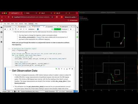
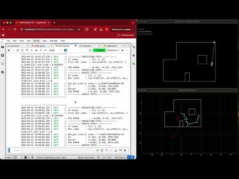
In the first video, we observe that without the Bayes filter, the odometry model (red) performs poorly in predicting the robot’s actual trajectory (green). This is evident from the significant discrepancy between the two paths. In contrast, the second video shows that applying the Bayes filter (blue) results in significantly improved position estimates. This improvement is highlighted by the close alignment between the blue and green trajectories on the trajectory plotter.

Without Bayes Filter

With Bayes Filter

Refrences

In Lab 10, I referenced Daria Kot's and Annabel Lian's webpages as well as Professor Helbling’s lecture slides for guidance on Bayes filter implementation in python. I also used ChatGPT to assist with text editing.