Lab 2
Objective
The goal of lab one was to begin using our first board peripheral, the IMU. We were also responsible for collecting our cars and recording a stunt.
Prelab
As the prelab exercise, we were responsible for familiarizing ourselves with the Sparkfun breakout board and the associated software library. Additionally we read the ICM-20948 datasheet to gain an understanding of the accelerometer gyroscope and magnetometer.
Accelerometer
I began by using the equations in lecture to convert the accelerometer data to pitch and roll. The equations could be found in the lecture slides as well as the example code provided in lecture 4. This made for a straightforward implementation process.
pitch_accel[valCount] = atan2(myICM.accX(),myICM.accZ())*180/M_PI;
roll_accel[valCount] = atan2(myICM.accY(),myICM.accZ())*180/M_PI;
To perform the sweep from -90 to 90 I attached the accelerometer to a box which I then rotated while collecting data. I performed this action for both pitch and roll yielding the following plots:
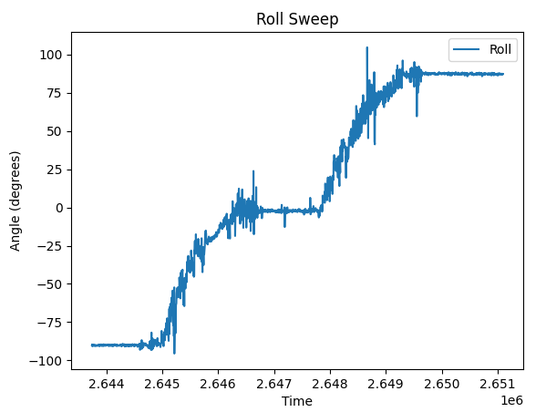
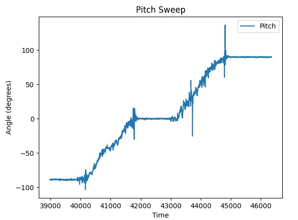
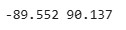
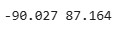
To improve the accuracy of my accelerometer I explored using 2 point calibration. However, in my measurements of two points, I found them to be close enough to -90 and 90 that I chose not to. Considering I was using a cardboard box as my means of measuring these angles I reasoned that considering the relative inaccuracy of the method, 2 point calibration would not yield a meaningful increase in accuracy and therefore was not a beneficial exercise.
Pitch:
 Roll:
Roll:
When holding the accelerometer in close proximity with the spinning motors of the car, the data didn’t appear to be very noisy.
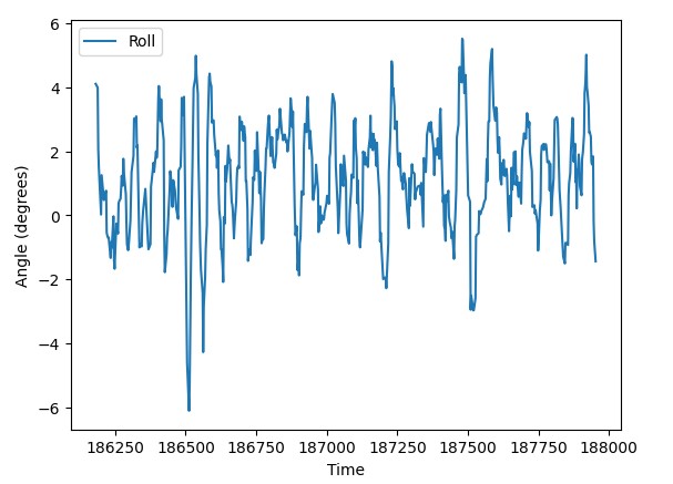
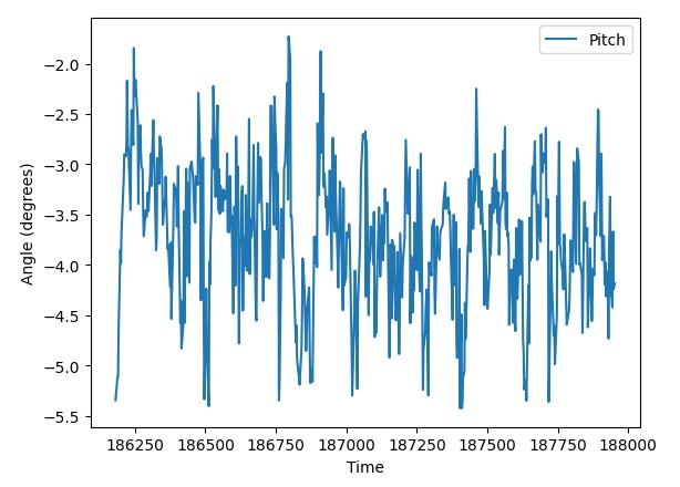 Although the data looks fairly noisy on the plot, the relative amplitude of the noise is pretty low, only drifting a few degrees from center in each direction.
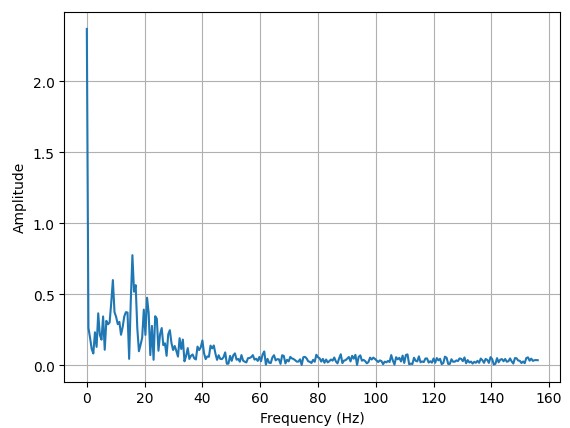
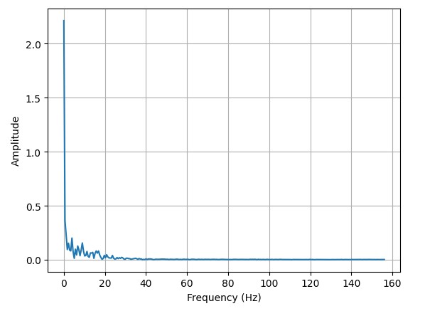
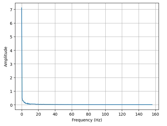
A fourier analysis was performed on the pitch and roll data yielding the following results:
Roll:
 Pitch:
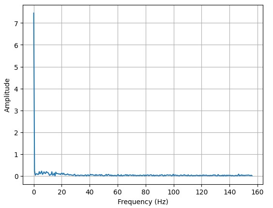 It can be observed that in both plots, most of the frequency composition is around the fundamental with a small peak around 15Hz on the roll plot. From this data, I reasoned that a good cutoff frequency would be 2Hz.
time = np.array(time_data) / 1000.0
sample_intervals = np.diff(time)
avg_sample_rate = 1 / np.mean(sample_intervals)
f = avg_sample_rate #Sampling Frequency
fc = 2 #Cutoff Frequency
alpha = (1/f)/((1/f)+(1/(2*np.pi*fc)))
print(alpha)
The above code was used to compute the alpha value considering the data, sampling rate and desired cutoff frequency. It yielded a value of 0.038. The equation used to calculate alpha is an adaptation of that of an RC low pass filter which we covered in lecture. In practice, the choice of alpha values informs how well your filtered data tracks the measured data. The benefit is that with the appropriately chosen value, it will mitigate the influence of noise on the output. However if the alpha value gets too small, meaning your cutoff frequency is very low, you risk filtering out the meaningful components of the data.
Roll:
 Pitch:
Above are the plots of the fourier analysis of the same pitch and roll data after it has been filtered. It can be observed that frequencies above the fundamental are being attenuated.
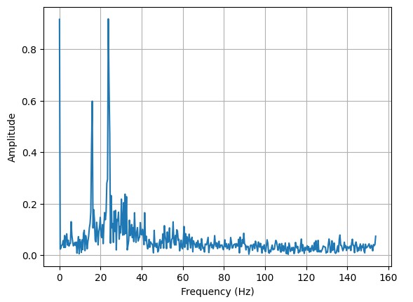
When introducing vibrational noise by gently hitting the table it yields the following fourier analyses.
Roll:
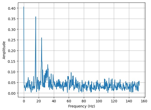 Pitch:
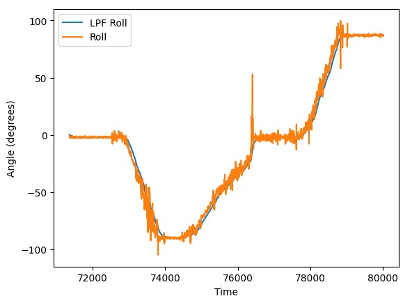
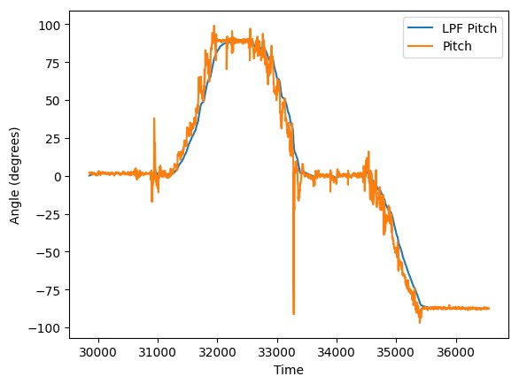
Below are examples of how the low pass filter approach works in practice. We can observe how the filtered data follows general the trend of the unfiltered data.
Gyroscope
Using the equations from lecture and the provided lecture 4 code I added pitch roll and yaw angle calculations that use gyroscope data.
if(counter == 0){
   dt = 0;
 }
 else{
   dt = (micros()-last_time)/1000000.;
 }
 last_time = micros();
 pitch_g = pitch_g + myICM.gyrY()*dt;
 roll_g = roll_g + myICM.gyrX()*dt;
 yaw_g = yaw_g + myICM.gyrZ()*dt;
 pitch_gyro[counter] = pitch_g;
 roll_gyro[counter] = roll_g;
 yaw_gyro[counter] = yaw_g;
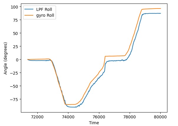
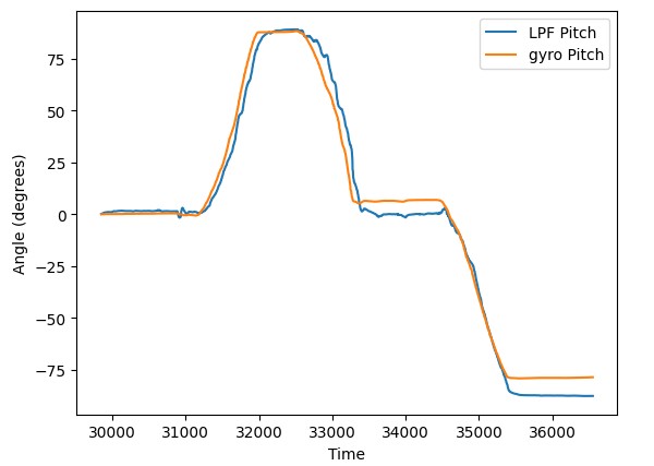
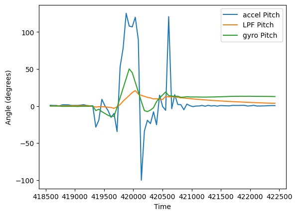
As we can observe in these plots, generally speaking, the gyro data and the filtered data follow very similar trends. This is a strong indication that we chose an appropriate cutoff frequency because gyro data is far less susceptible to noise than the accelerometer. However, We also see that the value at which the gyro and filtered accelerometer data settle on on the right of our graphs are different. This is a consequence of the gyro's susceptibility to drift. The values are supposed to be 90 degrees for roll and -90 degrees for pitch but in both cases the magnitude of the gyro data is observably larger. Because the the discrete integration approach used to gyro angle calculations, if we were to decrease the sampling rate, it only exacerbates the drift issues. As we can see below, in a relatively short time window one rapid rotation introduces a significant amount of drift in the gyro angle calculation when a 50 millisecond delay is included.
A method to capitalize on the minimal gyro noise and lack of accelerometer drift is a complementary filter approach. Using the formula outlined in the lecture slides I was able to implement a complementary filter that capitalizes on the best elements of both approaches.
comp_pitch[counter] = ((comp_pitch[counter - 1] + myICM.gyrY()*dt) * (1 - alpha)) + (pitch_accel[counter] * alpha);
 comp_roll[counter] = ((comp_roll[counter - 1] + myICM.gyrX()*dt) * (1 - alpha)) + (roll_accel[counter] * alpha);
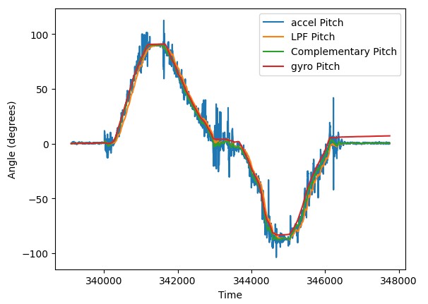 This plot demonstrates the benefits of the complementary filter approach. The output closely tracks the signal without being influenced by the quick vibrations associated with rotation. Furthermore, we can observe drift in the gyro data on the right of our graph; however, the complementary filter does not experience that drift and is able to return to 0. The output behavior is strongly influenced by the choice of alpha value which in this case I found experimentally.
Sample Data
In my implementation, due to issues with my computer crashing when trying to regular prints to serial, I didn't include any print statements in my main loop. I used a flag (GET_DATA) to toggle data collection on and off in loop via bluetooth commands. I created an if statement that collects data when it is available. I also include an else condition that is supposed to print "No Data Available." However this output was never displayed on the serial monitor. Because it was never entering the else condition we can reason that the IMU produces new values at a rate faster than the Artemis can read them in the loop.
void
loop()
{
   // Listen for connections
   BLEDevice central = BLE.central();
   // If a central is connected to the peripheral
   if (central) {
       Serial.print("Connected to: ");
       Serial.println(central.address());
       // While central is connected
       while (central.connected()) {
           // Send data
           write_data();
           // Read data
           read_data();
           if(myICM.dataReady()){
             myICM.getAGMT();
             if(GET_DATA){
                 ...
               }
           }
           else{
             Serial.println("No Data Available");
           }
       }
       Serial.println("Disconnected");
   }
}
For my data collection I chose to have each type of data stored in its own array. I had 9 arrays of floats and 1 array of unsigned long for my time stamps. I made the decision to use floats for data because I need the fractional information and unsigned long for the time stamps because it can reach larger values than int which has caused me issues previously. I chose multiple arrays because it made for easier parsing and data transmission. Considering that floats and unsigned long are 4 bytes, at each sample time step, I am storing 40 bytes of data. Assuming memory is being used for nothing else, this would enable me to take 9600 samples. Looking at the time stamp information on my transmitted data, I am able to collect 2780 samples in 8.642 seconds. My sample rate is ~321.68 samples/sec. Considering that I can collect a maximum of 9600 samples, I can collect data for ~29.84 seconds before running out of memory. By looking at the timestamps on the complementary filter plot it demonstrates that I can collect at least 5s worth of IMU data and send it over bluetooth.
Record a stunt!

Refrences
I used code from the scipy website to create my fourier plots. I used ChatGPT to help resolve some compilation issues I was having related to RAM and to write code to calculate sampling frequency. I utilized the example code associated with the lecture to convert accelerometer and gyro data to angles.