Lab 5
Objective
The lab 5 exercise was intended to help us gain experience with PID control. We were tasked with implementing position control using a P, PI, PD, or PID controller. As a 5000-level student, I needed to choose between PI and PID. The ultimate goal was to use ToF data to compute an error used to assess how far we were from our setpoint and let that value inform our control to minimize oscillation.
Prelab
An essential part of this lab was creating a robust debugging protocol. This included implementing a start input transmitted to the Artemis over Bluetooth and a PID duration limit responsible for stopping the PID after a specified duration to prevent our car from running off uncontrollably. Additionally, to help analyze behavior and performance, it’s important that we transmit important data back to our computer for analysis on Jupyter. This data includes time stamps, ToF data, and PWM output.
The following method was used to implement the start and time constraints on PID control. I use a bluetooth command to set a flag high which triggers PID to begin running in loop. This command takes in k values and well as PWM minimum and maximum constraints and assigns them to the global variables used to inform PID. Based on the while condition, PID can only run for 5 seconds contingent on the flag having been set high from the command, and bluetooth being connected.
void
handle_command()
{
    switch (cmd_type) {
        case PID:
            float Kp, Ki, Kd, PWM_MIN, PWM_MAX;

            success = robot_cmd.get_next_value(Kp);
            if (!success) return;

            success = robot_cmd.get_next_value(Ki);
            if (!success) return;

            success = robot_cmd.get_next_value(Kd);
            if (!success) return;

            success = robot_cmd.get_next_value(PWM_MIN);
            if (!success) return;

            success = robot_cmd.get_next_value(PWM_MAX);
            if (!success) return;

            PID_flag = true;
            break;

void
loop()
{
    BLEDevice central = BLE.central();

    if (central) {
        while (central.connected()) {
            write_data();

            read_data();

            start_time_1 = millis();
            while (millis() - start_time_1 < 5000 && PID_flag && central.connected()) {
              sensor2.startRanging();
              if(sensor2.checkForDataReady()){

            ###Perform PID###

            PID_flag = false;
            }

            ###Send data over bluetooth###
        }
        Serial.println("Disconnected");
    }
}
Data transmission back to my computer via bluetooth was performed using the same methods as previous labs.
PID
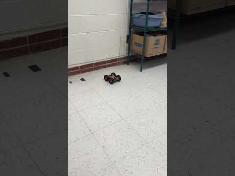
To benchmark the performance of our PID controller, we strived to have our robot drive as fast as possible towards the wall and stop 1ft (304mm) away using ToF data to inform our PID or PID variation. Additionally, our controller should be resistant to variable conditions like initial distance from the wall and surface texture. In Lab 3, I used my ToF sensors set in the short mode because of the shorter-ranging time and resistance to ambient light. However, considering that we wanted our controller to operate at a wide range of start distances from the wall, lab 3 demonstrated that it only yields reasonable results at less than a meter. I decided to switch to long range, which produces reasonable results until around 4m. I choose to start with a small proportional gain of 0.001. Considering the discussion of PID in class, the first heuristic tuning method recommended beginning with a small Kp value. Considering the magnitude of my errors and my PWM output value output range, this value would produce conservative PID outputs. Considering I initially did not understand the controller's performance, choosing a smaller kp value generally resulted in a less aggressive controller. With our ToF sensors, we can adjust the timing budget and inter-measurement period. The timing budget can be set as low as 33ms in long mode. Faster updates have the potential to improve the performance of the system. I chose to assess how well my controller performed in the default mode and use those results to inform whether increasing the ToF sampling rate would be beneficial. I also chose to use the default integration time and decide if adjustment was necessary.
Considering that I would have to do at least PI control, I began by implementing the entire PID controller.
integral += error * dt;

double derivative = (error - last_error) / dt;
last_error = error;

double pid_output = Kp * error + Ki * integral + Kd * derivative;

if(pid_output >= 0){
  #Spin motors forward
}
else{
  #Spin motors backwards
}
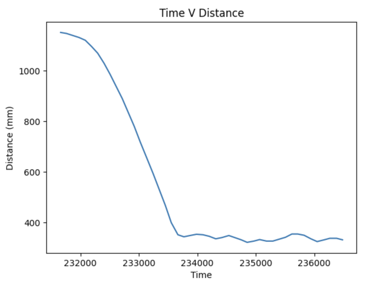
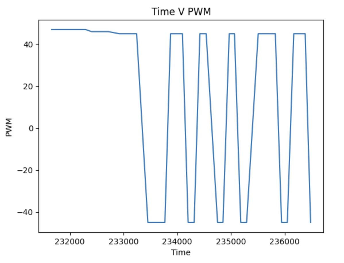
I created my command to send kp, ki, and kd values over Bluetooth to facilitate rapid experimentation. Additionally, with the whole PID controller integrated, I could explore various configurations by setting the unwanted k terms to 0. I chose to begin with PID immediately. I tuned my PID controller using the heuristic one covered in lecture 7. I set kp to 0.001, increased kd until oscillation, then decreased it by a factor of 2. I then increased kp until overshoot, reduced by a factor of 2. I then increased ki until oscillation. I increased kd until oscillation then decreased it by a factor of 2. I increased kp until overshoot, then reduced it by 2. After these two iterations, I landed on kp = 0.003, ki = 0.0000001, and kd = 0.0007. This controller makes a fairly conservative approach to the setpoint at which we observe small oscillations both in the video and on the plot. On the PWM plot at oscillation we observe the jump between negative and positive values across the deadband whose magnitude is informed by the lower limit that my PWM value is constrained to. This lower limit is the minimum PWM value to create movement from a stop.
It can be good practice to low-pass filter the derivative term or, as previously discussed, increase the sample rate, but considering the performance of the default settings and unfiltered derivative, I decided it was unnecessary for this case. In the default case the sampling frequency was very low, only 7Hz found using this code:
print((len(distance_data)/(time_data[-1] - time_data[0]))* 1000)
Additionally, considering that I constrained my maximum PWM value to 85 and designed a conservative controller my maximum linear speed was also low, 0.27m/s found using this code:
speeds = np.diff(distance_data) / np.diff(time_data)
max_speed = np.max(speeds)
print(max_speed)
Extrapolation
Following reasonable PID performance, the next step was experimenting with extrapolation before exploring Kalman Filtering in lab 7. The first step was to pull the PID portion out of my loop, which would only update the PID output when new data was available. This modification causes the PID control to run faster than the data sampling rate. In an ideal case I don’t believe this should have any impact on the system. The integral is resistant to time scaling, and the summed error over smaller intervals should be equal to that of the larger interval. Furthermore, when no new data is available the (previous error - error) should yield zero for the derivative term. In practice, this method yielded noticeably worse results, as demonstrated in this video:
To add a predictive element to PID, I use linear extrapolation using the slope between the last two measured points to predict the distance at the current time step. It doesn't begin PID until at least two values have been measured and extrapolation can begin. This is done using this code:
start_time_1 = millis();
while (millis() - start_time_1 < 5000) {

    sensor2.startRanging();
    unsigned long now = millis();
    float currentDistance = 0.0;

    if (measure_index < 2) {
        if (sensor2.checkForDataReady()){
            currentDistance = sensor2.getDistance();
            measured_distances[measure_index] = currentDistance;
            measured_times[measure_index] = now;
            measure_index++;
        }
    }
    else {
        if (sensor2.checkForDataReady()){
            currentDistance = sensor2.getDistance();
            measured_distances[measure_index] = currentDistance;
            measured_times[measure_index] = now;
            measure_index++;
        }
        else {
            if (measure_index >= 2) {
                unsigned long t_last = measured_times[measure_index - 1];
                unsigned long t_prev = measured_times[measure_index - 2];
                float d_last = measured_distances[measure_index - 1];
                float d_prev = measured_distances[measure_index - 2];

                if (t_last > t_prev) {
                    float slope = (d_last - d_prev) / (float)(t_last - t_prev);
                    unsigned long dt = now - measured_times[measure_index - 1];
                    currentDistance = d_last + slope * dt;
                } else {
                    currentDistance = d_last;
                }
            }
        }
    }

    if(measure_index > 2){

      ###Perform PID with currentDistance###

      index++;

      sensor2.clearInterrupt();
      sensor2.stopRanging();
    }
}
Below, you can see the plot of the predicted data vs. the measured data. We can observe that they generally follow the same trend.
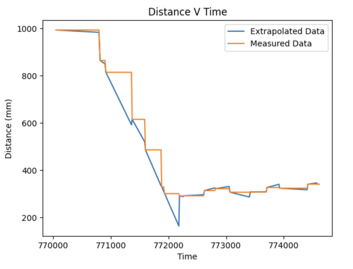
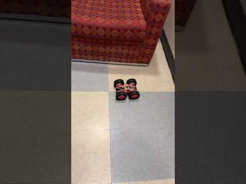
My car would consistently overshot my setpoint and then settled at a point behind it. By retuning my PID controller for the extrapolation, I was able to get reasonably good results with kp = 0.01, ki = 0.0000003, and kd = 0.0008.
Although I was able to get it to work well, there is likely some benefit to increasing the sampling rate to mitigate the observable drift that occurs between measured and predicted data seen as vertical lines on the extrapolated data plot.
Tasks for 5000-level students
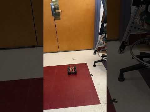
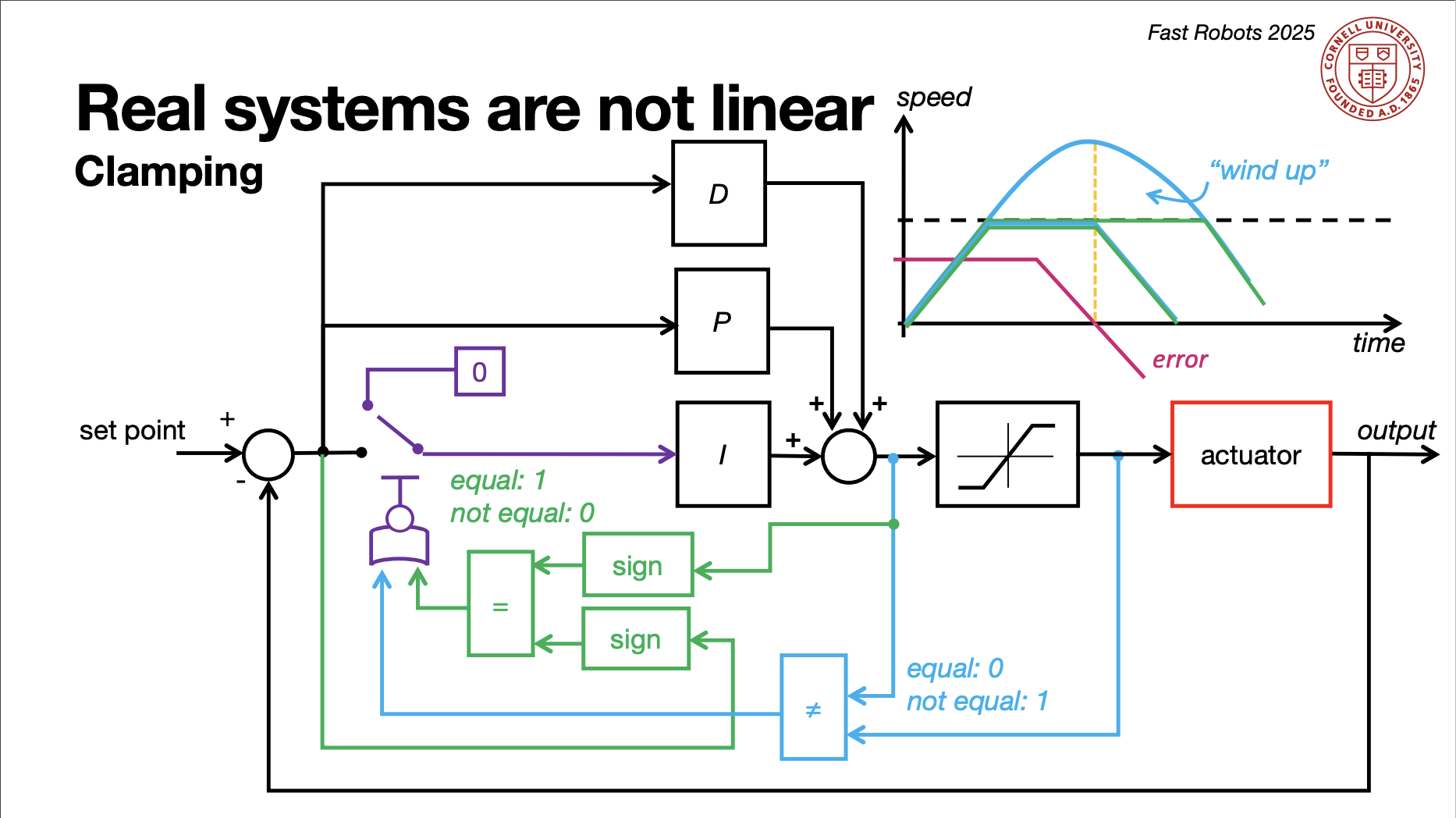
In the final part of this lab, we implemented wind up protection for the integrator which is a critical feature of any robust PID controller. Wind up protection works by clamping the integrator term to prevent it from accumulating excessive error when the error persists for an extended period. This limitation is significant because without it, the integrator could drive the system into an excessive overshoot, making the time to stabilization longer. By limiting the integrator's influence, wind up protection enables the plant to stabilize more quickly, even under prolonged error conditions. Windup protection was added using this code:
if(error > 0 && pid_output > 0 && pid_output + PWM_MIN == PWM_MAX || error < 0 && pid_output < 0 && pid_output - PWM_MIN == -PWM_MAX){
  integral = integral;
} else {
  integral += error * dt;
}
This method of windup protection was inspired by the diagram provided in lecture 8.
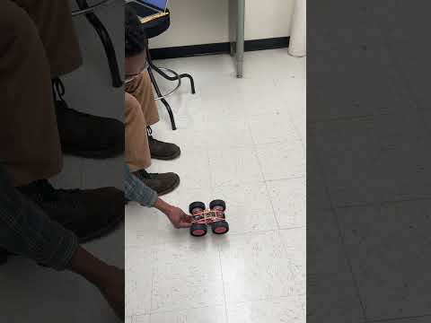
This fairly simple modification allows the car to become resistant to wind up, as demonstrated in this video.
Refrences
In lab 5 I referenced Nila’s webpage to guide formatting and content. Throughout this lab I consulted other students in the course about various elements of the assignment. These students included Annabel Lian, Becky Lee, Aidan McNay, and Aidan Derocher. I used ChatGPT to help with debugging as well as some code generation for plotting data and elements of PID implementation and extrapolation.