Return to Main Page

Lab 7

Objective

The goal of Lab 7 is to implement Kalman Filtering to supplement our Time-of-Flight (ToF) sensor data with predictive estimates, facilitating faster performance.

Estimate drag and momentum

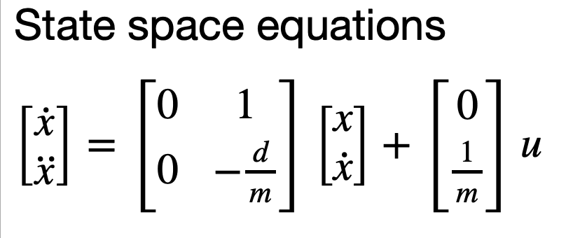
We first needed to estimate the drag and momentum terms for our A and B matrices to create our Kalman filter. This was achieved using a step response. I drove my car towards the wall at a constant PWM input of 175 and logged the ToF distance values. A critical part of this step response test was that the car ran long enough for it to reach a steady state, which is the point where its speed is constant. The mass (m) and drag (d) were found using these equations.

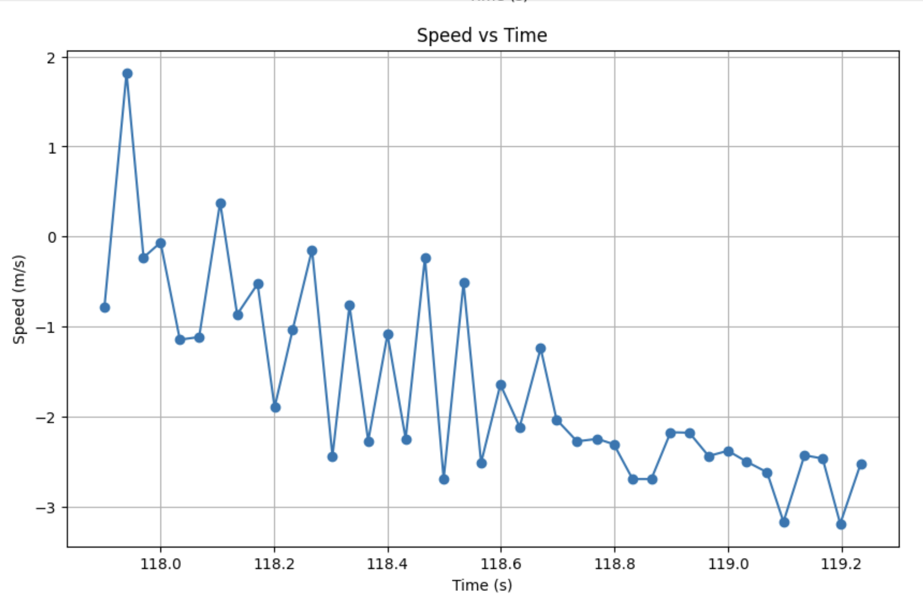
For my step response u(t), my PWM was 175, which is ~68%. I use active braking to prevent my car from hitting the wall, but I make sure not to include the ToF data from the active braking period.

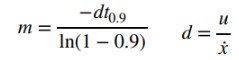
Below is a graph of my ToF data, speed, and PWM vs. time.

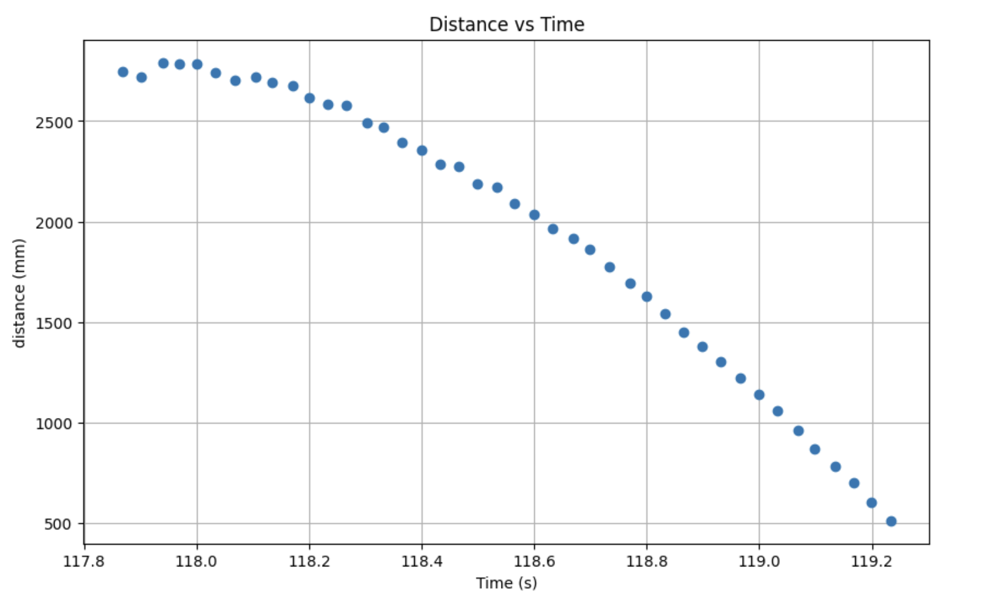
As we can observe from the plots, the distance data is consistent with what one would expect from a step response. However, the speed data is very noisy on the speed vs. time plot. Considering how noisy the data is, it’s difficult to choose where to measure 90% rise time and speed at 90% rise time. To help address this, I fitted an exponential curve to my data.

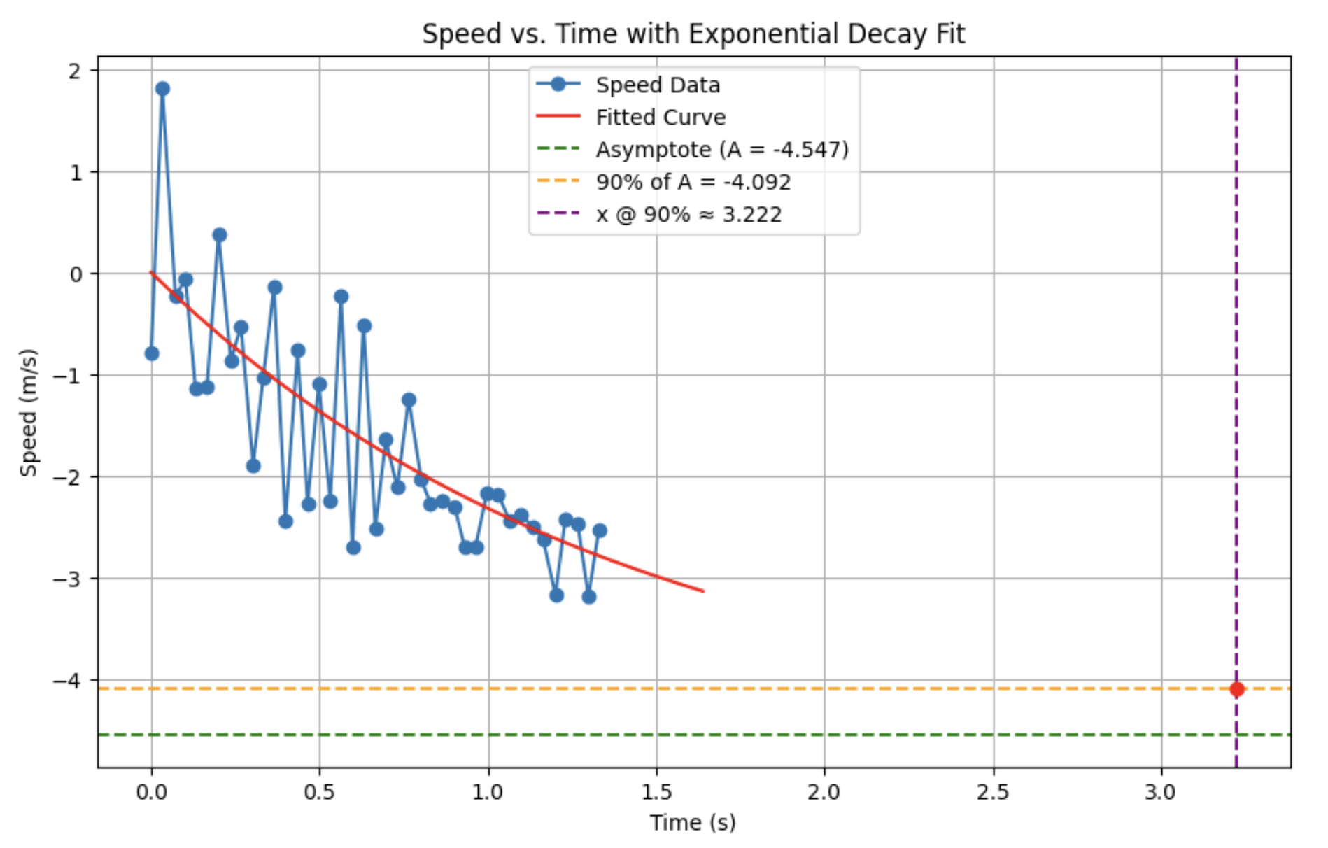
As we can observe from this plot, the calculated parameters don’t provide meaningful information. In the distance vs. time plot, we see a linear region corresponding to the steady state speed near the end of the plot.

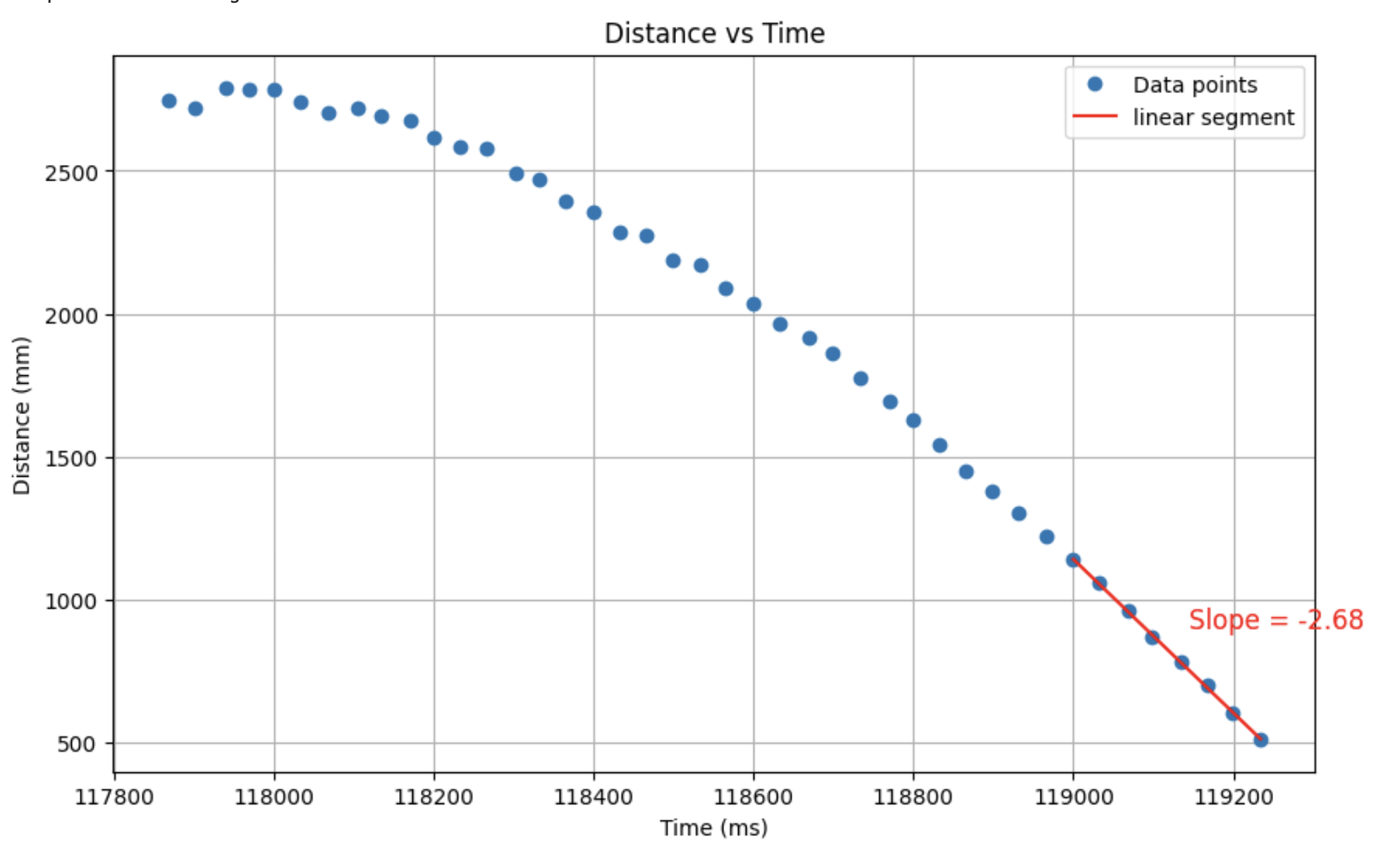
I assumed that this constituted a steady state and, in turn, adjusted the parameters of my exponential fit to yield a curve that was more consistent with that observation. From this plot, I found my rise time and speed at 90% rise time.

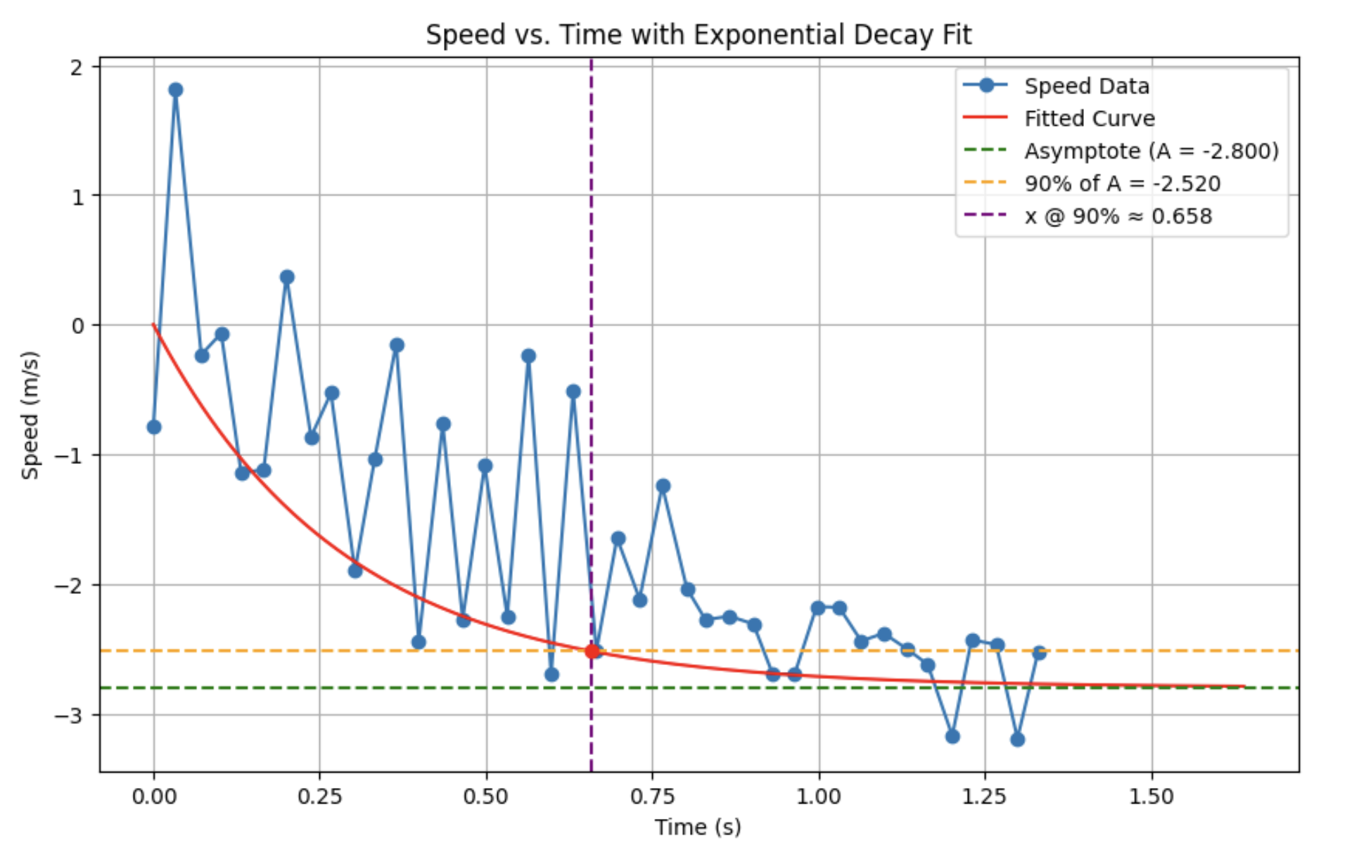
Using the values from this plot I calculated m and d using this code:

d = 1/2.52   # damping coefficient
m = (-0.658 * d) /math.log(1-0.9)   # mass

Referencing the code from the lab assignment, I discretized my A and B matrices so that they could be used to simulate our Kalman filter in Python. To find my Delta_T value, I found the average time between measurements in my step response data. Considering that time is collected and transmitted in milliseconds, I normalized the values such that time would be expressed in seconds for my Kalman filter calculations. Before we could run our simulation, we needed to find our sigma 1, sigma 2, and sigma 3. The first two correspond to process noise, and sigma 3 is the sensor noise. I was able to find sigma 3 by performing stationary ToF data acquisition with the motors spinning. I then took the standard deviation of the data, which returned a value of 5mm. Sigma 1 and 2 are more difficult to compute, and it was recommended to me by a TA during office hours to start with a value of 10 and adjust to reach the desired performance. Generally speaking, increasing Sigma 1 and 2 decreases your trust in the model while lowering it means increased trust. Using the following code, I implemented Kalman filtering in Python. The code is heavily inspired by the implementation in the lecture and the lab 7 assignment.

Delta_t = 0.0333

d = 1/2.52   # damping coefficient
m = (-0.658 * d) /math.log(1-0.9)   # mass

A = np.array([[  0  ,  1   ],
              [  0  , -d/m ]])

B = np.array([[  0  ],
              [ 1/m ]])

Ad = np.eye(n) + Delta_t * A
Bd = Delta_t * B
C = np.array([[1,0]])
x = np.array([[distance[0]], [0]])
sigma_1 = 23
sigma_2 = 23
sigma_3 = 5
Sigma_u=np.array([[sigma_1**2,0],[0,sigma_2**2]])
Sigma_z=np.array([[sigma_3**2]])

def kf(mu,sigma,u,y):

    mu_p = A.dot(mu) + B.dot(u) 
    sigma_p = A.dot(sigma.dot(A.transpose())) + Sigma_u

    sigma_m = C.dot(sigma_p.dot(C.transpose())) + Sigma_z
    kkf_gain = sigma_p.dot(C.transpose().dot(np.linalg.inv(sigma_m)))

    y_m = y-C.dot(mu_p)
    mu = mu_p + kkf_gain.dot(y_m)    
    sigma=(np.eye(2)-kkf_gain.dot(C)).dot(sigma_p)

    return mu,sigma

sigma = np.array([[20**2, 0], [0, 10**2]])

kf_data = []

for i in range(0, len(time)):
    x, sigma = kf(x, sigma, 1, distance[i])
    kf_data.append(x[0])

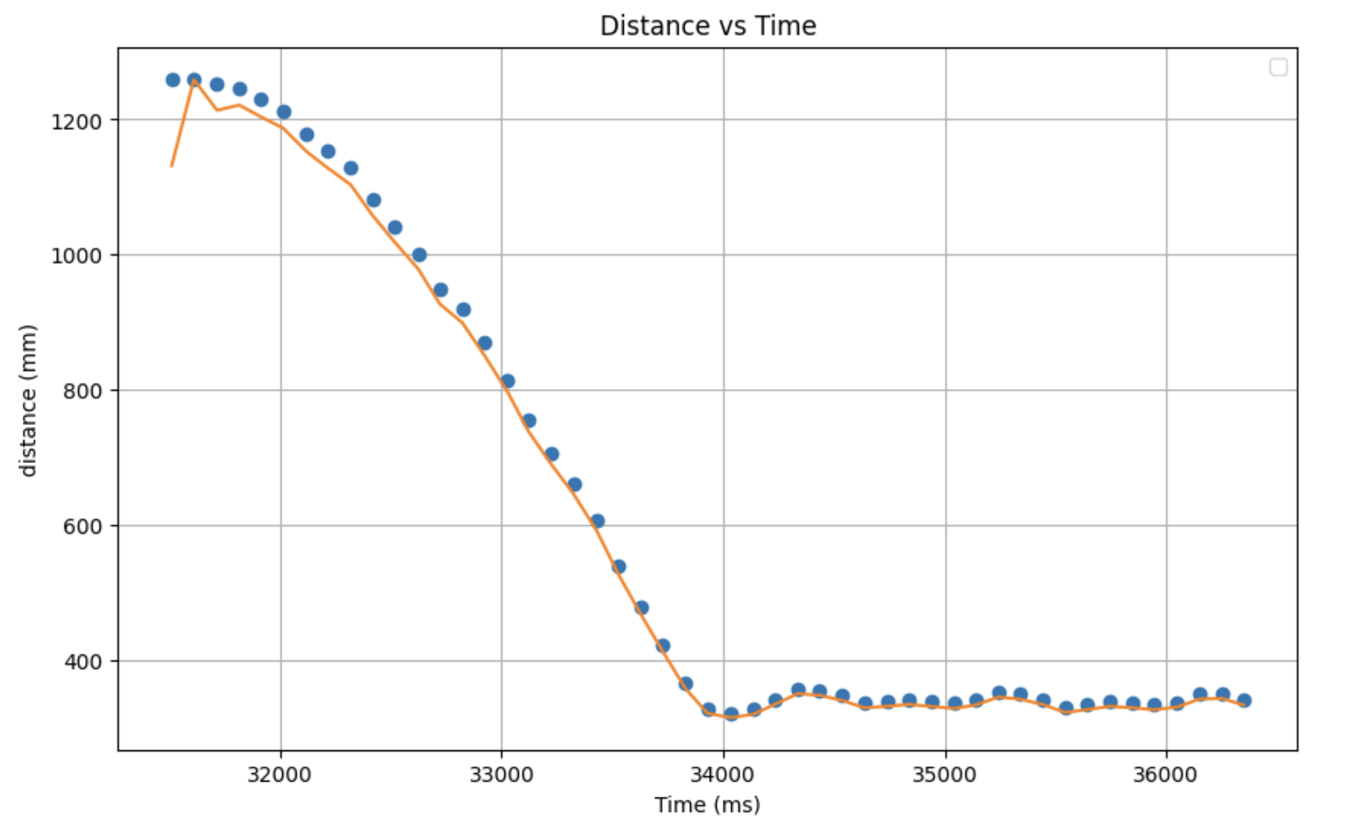
When run on my step response data it returned the following plot:

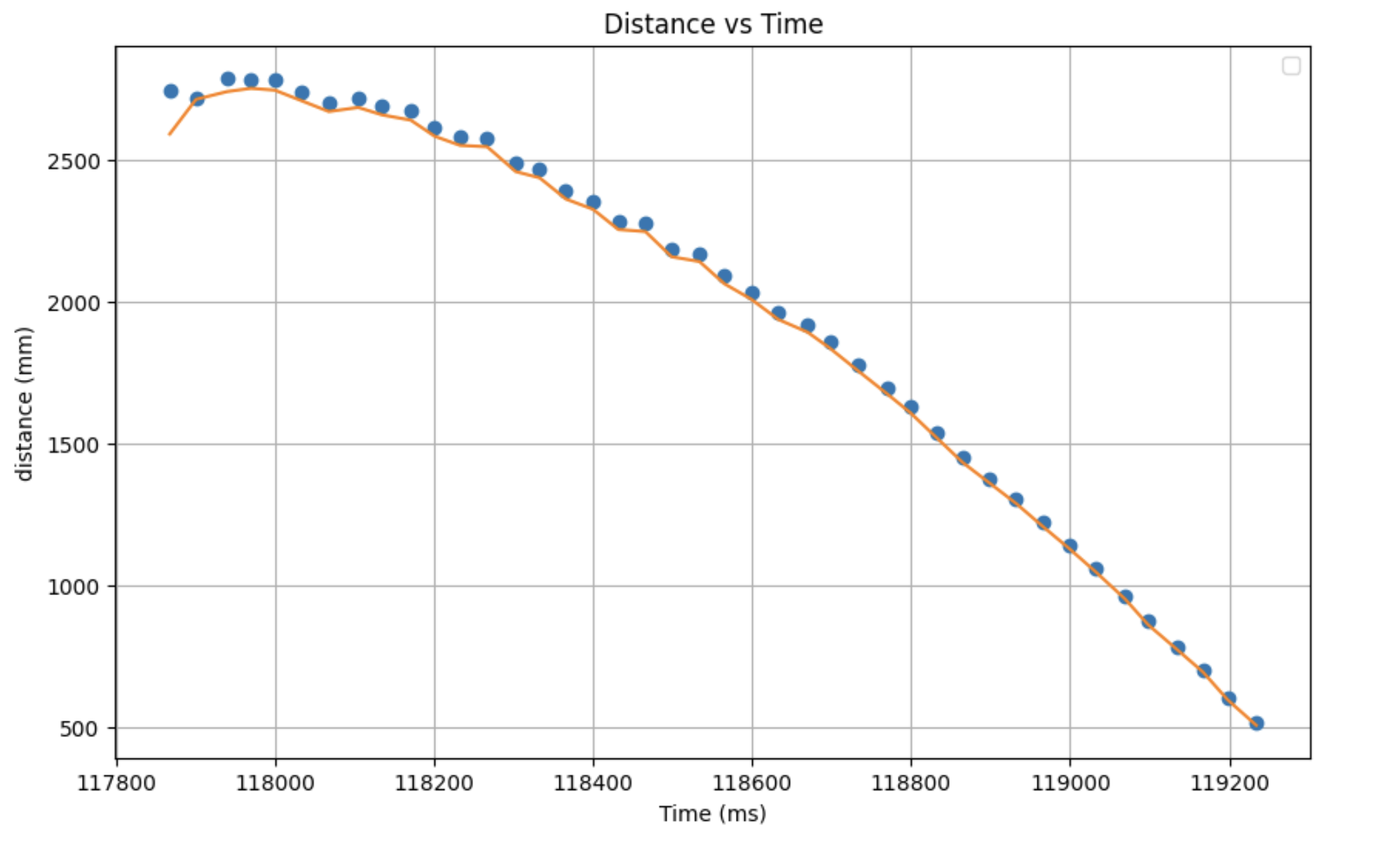
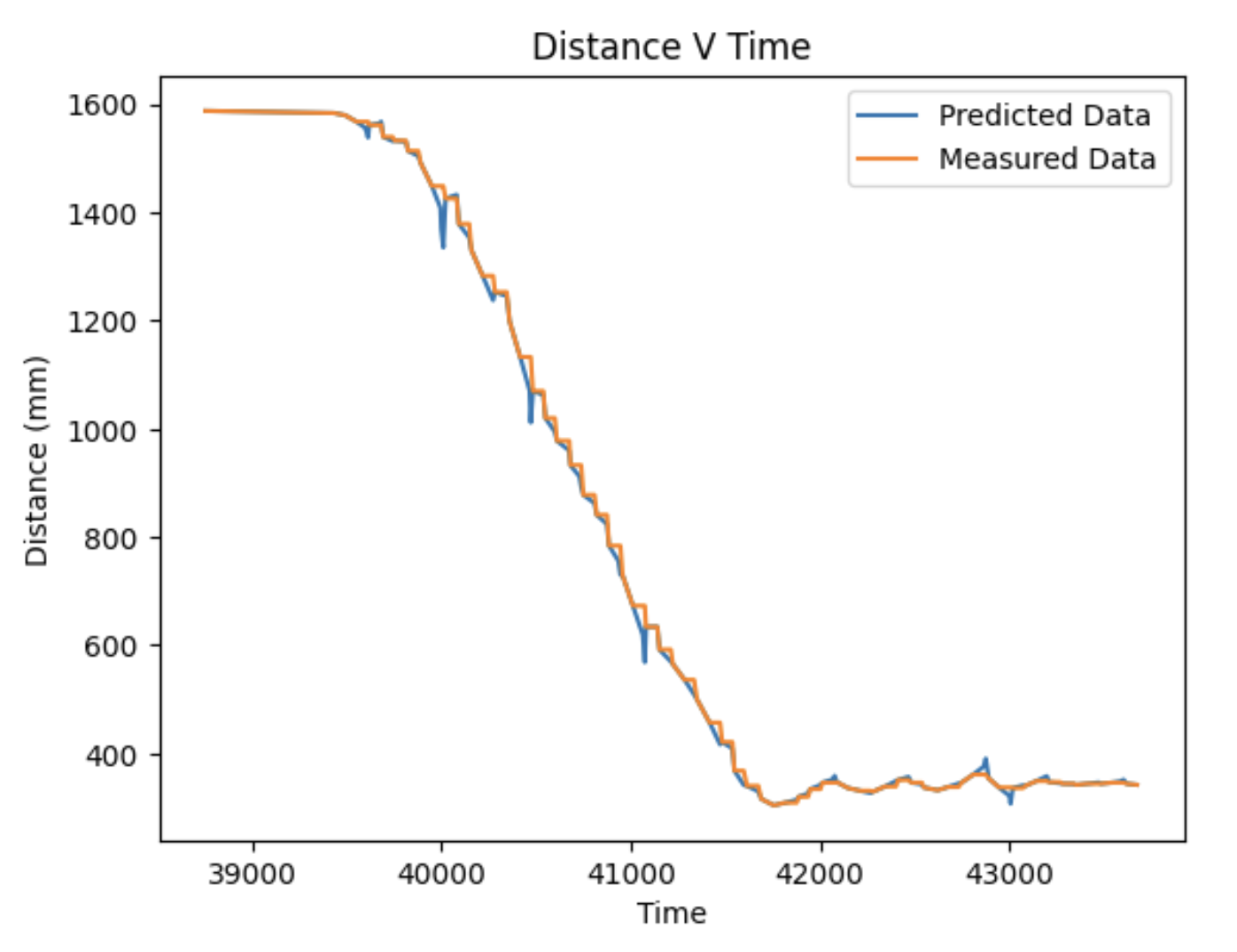
I increased the values of sigma 1 and sigma 2 from 10 to 23 to get the predictions to better match the measured values from the ToF. After successfully fitting the Kalman filter to my step response data, I used the same code to fit the Klaman filter to some of my recorded PID data from lab 5, yielding the following plot.

Having verified the functionality of my implementation in simulation, the last step of the lab was to implement Kalman filtering on the car. The last step was to implement the Kalman filter function in Arduino. This was done using this code, which closely resembles the Python implementation.

const float Delta_t = 13.145;

float d = 1 / 2.52;
float m = ((-0.658 * 1000 * d) / log(1 - 0.9));  

Matrix<2,2> A = {
 0,   1,
 0,  -d/m
};

Matrix<2,1> B = {
 0,
 1/m
};

Matrix<2,2> I = {
 1, 0,
 0, 1
};

Matrix<2,2> Ad = I + Delta_t * A;

// Bd = Delta_t * B
Matrix<2,1> Bd = Delta_t * B;

Matrix<1,2> C = {
 1, 0
};

Matrix<2,1> x = {
 distance0,
 0
};

float sigma_1 = 30;
float sigma_2 = 30;
float sigma_3 = 5;

Matrix<2,2> Sigma_u = {
 sigma_1 * sigma_1,          0,
 0,           sigma_2 * sigma_2
};

Matrix<1,1> Sigma_z = {
 sigma_3 * sigma_3
};

Matrix<2,1> mu;            
Matrix<2,2> sigma = { 1, 0,
                     0, 1 };

Matrix<1,1> u;

Matrix<1,1> y ;
Matrix<1,1> y_pred;
Matrix<2,1> mu_p;

void kf(const Matrix<1,1>& u, const Matrix<1,1>& y, Matrix<2,1>& mu, Matrix<2,2>& sigma) {
   Matrix<2,1> mu_p = Ad * mu + Bd * u;

   Matrix<2,2> sigma_p = Ad * sigma * (~Ad) + Sigma_u;

   Matrix<1,1> sigma_m = C * sigma_p * (~C) + Sigma_z;

   Matrix<1,1> sigma_m_inverse = Inverse(sigma_m);

   Matrix<2,1> kkf_gain = sigma_p * (~C) * sigma_m_inverse;

   Matrix<1,1> y_m = y - (C * mu_p);

   mu = mu_p + kkf_gain * y_m;

   Matrix<2,2> I = { 1, 0, 0, 1 };
   sigma = (I - kkf_gain * C) * sigma_p;
}

I then modify my Lab 5 linear extrapolation such that in instances where data is available the measured values are passed into the the kf function. This is achieved in arduino using this code:

case PID:
           float Kp, Ki, Kd, PWM_MIN, PWM_MAX;

           success = robot_cmd.get_next_value(Kp);
           if (!success) return;

           success = robot_cmd.get_next_value(Ki);
           if (!success) return;

           success = robot_cmd.get_next_value(Kd);
           if (!success) return;

           success = robot_cmd.get_next_value(PWM_MIN);
           if (!success) return;

           success = robot_cmd.get_next_value(PWM_MAX);
           if (!success) return;

           start_time_1 = millis();
           sensor2.startRanging();

           u(0,0) = 1;

           while (millis() - start_time_1 < 5000) {  // Run for 5 seconds
               unsigned long now = millis();
               float currentDistance = 0.0;
               bool measurementAvailable = sensor2.checkForDataReady();
               if (measurementAvailable) {
                   float measuredValue = sensor2.getDistance();

                   # If the filter hasn't been initialized, use the first measurement.
                   if (!kalman_initialized) {
                       mu(0,0) = measuredValue;  // Initialize position
                       mu(1,0) = 0;              // Assume initial velocity = 0
                       kalman_initialized = true;
                   } else {
                       # With filter already initialized, perform a full Kalman filter update.
                       y(0,0) = measuredValue;
                       u(0,0) = abs((float)pwm_vals[index - 1])/175;
                       kf(u, y, mu, sigma);
                   }
                   measured_distances[measure_index] = measuredValue;
                   measured_times[measure_index] = now;
                   sensor2.clearInterrupt();
                   measure_index++;
               }
               else {
                   # No new measurement available.
                   if (kalman_initialized) {
                     u(0,0) = abs((float)pwm_vals[index - 1]) / 175;
                     // Prediction step only:
                     Matrix<2,1> mu_p = Ad * mu + Bd * u;
                     Matrix<2,2> sigma_p = Ad * sigma * (~Ad) + Sigma_u;
                     mu = mu_p;
                     sigma = sigma_p;
                   }
               }

               # Do not run PID control until the filter has been initialized.
               if (!kalman_initialized) {
                   sensor2.clearInterrupt();
                   continue; // Skip PID until we have at least one measurement.
               }

               # Use the estimated position as the current distance.
               currentDistance = mu(0,0);
               distance = currentDistance;

               distances[index] = currentDistance;
               time_stamps[index] = now;

               ### Perform PID based on distance. ###
               index++;
           }
            ### Transmit Data ###
           break;

Considering that the loop is running faster than the ToF frequency, there are cases where no data is available, and predictions are made using the Kalman filter. These predictions are generated using this equation found on the lecture 14 slides:

This predictive measurement approach worked well, as demonstrated by this plot which displays both Kalman filter predicted data and measured data against time.

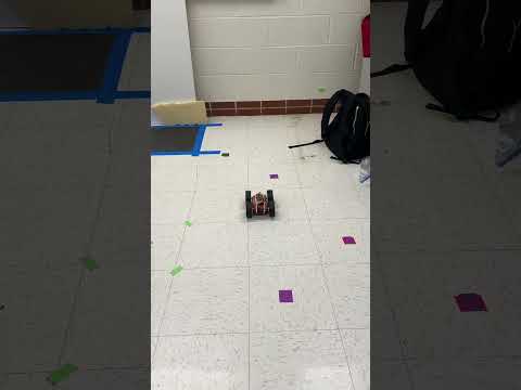
In this case the PID worked well with minimal overshoot and small oscillations around the set point using the same kp, ki, and kd terms as lab 5. Here is the video demonstrating its functionality:

Refrences

In lab 7 I consulted other students in the course about various elements of the assignment. These students included Annabel Lian, Becky Lee, and Akshati Vaishnav. I also referenced Stephan Wagner and Wenyi Fu's webpages. I used ChatGPT to help with debugging as well as some code generation for plotting data and elements of Kalman filter implementation.