Lab 9
Objective
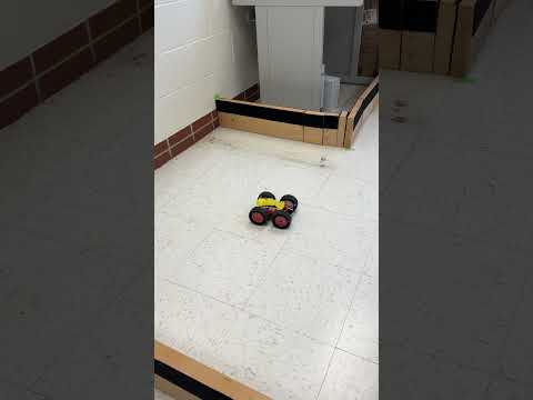
In Lab 9, we were tasked with mapping a static room using our robot. To generate this map, we placed the robot at several marked locations and had it rotate in place while collecting data from its Time of Flight (ToF) sensor. For the rotation mechanism, we had the option to use either open-loop control or a PID controller. After gathering angular and distance measurements, we used transformation matrices to convert the data into Cartesian coordinates, allowing us to construct a 2D representation of the environment.
Control
For rotation, I chose to use the orientation PID controller implemented in Lab 6. During a full rotation, the robot takes 15 measurements at 24-degree increments. Leveraging the same Bluetooth PID flag mechanism used in Lab 6, I modified the control loop to cycle through each setpoint and collect distance data. At each setpoint, the robot recorded 10 distance measurements along with the corresponding DMP-reported yaw angle. Given the inherent noise present in both the ToF and DMP sensors, I determined that averaging multiple readings at each point would improve the accuracy of the final map.
void loop() {
   BLEDevice central = BLE.central();
   if (central) {
       while (central.connected()) {
           write_data();
           read_data();


           if (PID_flag) {
               unsigned long stabilizationStart = millis();
               while (millis() - stabilizationStart < 2000) {
                   icm_20948_DMP_data_t dummyData;
                   myICM.readDMPdataFromFIFO(&dummyData);
                   delay(5);
               }


               start_time_1 = millis();
               bool yaw_offset_set = false;
               double yaw_offset_deg = 0.0;
               sensor2.startRanging();


               static int distance_count = 0;
               static int last_stage = -1;


               while (millis() - start_time_1 < 45000 && PID_flag && central.connected()) {
                   icm_20948_DMP_data_t dmpData;
                   myICM.readDMPdataFromFIFO(&dmpData);
                   if ((myICM.status == ICM_20948_Stat_Ok) ||
                       (myICM.status == ICM_20948_Stat_FIFOMoreDataAvail)) {
                       if ((dmpData.header & DMP_header_bitmap_Quat9) > 0) {
                           double q1 = ((double)dmpData.Quat9.Data.Q1) / 1073741824.0;
                           double q2 = ((double)dmpData.Quat9.Data.Q2) / 1073741824.0;
                           double q3 = ((double)dmpData.Quat9.Data.Q3) / 1073741824.0;
                           double q0 = sqrt(1.0 - ((q1 * q1) + (q2 * q2) + (q3 * q3)));
                           double yaw = atan2(2.0 * (q0 * -q3 + q1 * q2), 1.0 - 2.0 * ((q1 * q1) + (q3 * q3)));
                           double current_yaw_deg = yaw * 180.0 / M_PI;
                           if (current_yaw_deg < 0) {
                               current_yaw_deg += 360;
                           }


                           if (!yaw_offset_set) {
                               yaw_offset_deg = current_yaw_deg;
                               yaw_offset_set = true;
                           }


                           double yaw_relative = current_yaw_deg - yaw_offset_deg;
                           while (yaw_relative > 180) yaw_relative -= 360;
                           while (yaw_relative < -180) yaw_relative += 360;


                           unsigned long pid_elapsed = millis() - start_time_1;
                           int stage = pid_elapsed / 3000;
                           if (stage > 14) stage = 14;


                           double setpoints[15] = {0.0, 24.0, 48.0, 72.0, 96.0, 120.0, 144.0, 168.0, 192.0, 216.0, 240.0, 264.0, 288.0, 312.0, 336.0};
                           double setpoint = setpoints[stage];
                           if (setpoint > 180) setpoint -= 360;


                           double error = yaw_relative - setpoint;
                           while (error > 180) error -= 360;
                           while (error < -180) error += 360;


                           unsigned long now = millis();
                           double dt = (now - last_time) / 1000.0;
                           if (dt <= 0) dt = 0.001;
                           if (dt > 1) dt = 0.0001;
                           last_time = now;


                           if (dt == 0.0001) derivative = 0;
                           else derivative = (error - last_error) / dt;
                           last_error = error;


                           double pid_output = Kp * error + Ki * integral + Kd * derivative;
                           double pid_pwm = PWM_MIN + pid_output;


                           if (!((error > 0 && pid_output > 0 && pid_output + PWM_MIN == PWM_MAX) ||
                                 (error < 0 && pid_output < 0 && pid_output - PWM_MIN == -PWM_MAX))) {
                               integral += error * dt;
                           }


                           pid_pwm = constrain(pid_pwm, PWM_MIN, PWM_MAX);
                           int pwmValue = (int) pid_pwm;


                           if (fabs(error) < 2.0) {
                               analogWrite(AIN1, 0);
                               analogWrite(AIN2, 0);
                               analogWrite(BIN1, 0);
                               analogWrite(BIN2, 0);


                               // Reset distance count for new stage
                               if (stage != last_stage) {
                                   distance_count = 0;
                                   last_stage = stage;
                               }


                               if (distance_count < 10 && sensor2.checkForDataReady()) {
                                   last_distance = sensor2.getDistance();
                                   distances[index_1] = last_distance;
                                   yaws[index_1] = yaw_relative;
                                   sensor2.clearInterrupt();
                                   Serial.print("Distance ");
                                   Serial.print(distance_count + 1);
                                   Serial.print(": ");
                                   Serial.print(last_distance);
                                   Serial.println(" mm");
                                   distance_count++;
                                   index_1++;
                               }
                           } else {
                               if (pid_output >= 0) {
                                   analogWrite(AIN1, 0);
                                   analogWrite(BIN1, 0);
                                   analogWrite(AIN2, (int)(1.25 * pwmValue));
                                   analogWrite(BIN2, (int)(1.35 * pwmValue));
                                   pwm_vals[index_1] = pwmValue;
                               } else {
                                   analogWrite(AIN2, 0);
                                   analogWrite(BIN2, 0);
                                   analogWrite(AIN1, (int)(1.2 * pwmValue));
                                   analogWrite(BIN1, (int)(1.25 * pwmValue));
                                   pwm_vals[index_1] = -pwmValue;
                               }
                           }
                       }
                   }
               }


               sensor2.stopRanging();

               ###Transmit data###

               PID_flag = false;
               index_1 = 0;
           }
       }
       Serial.println("Disconnected");
   }
}
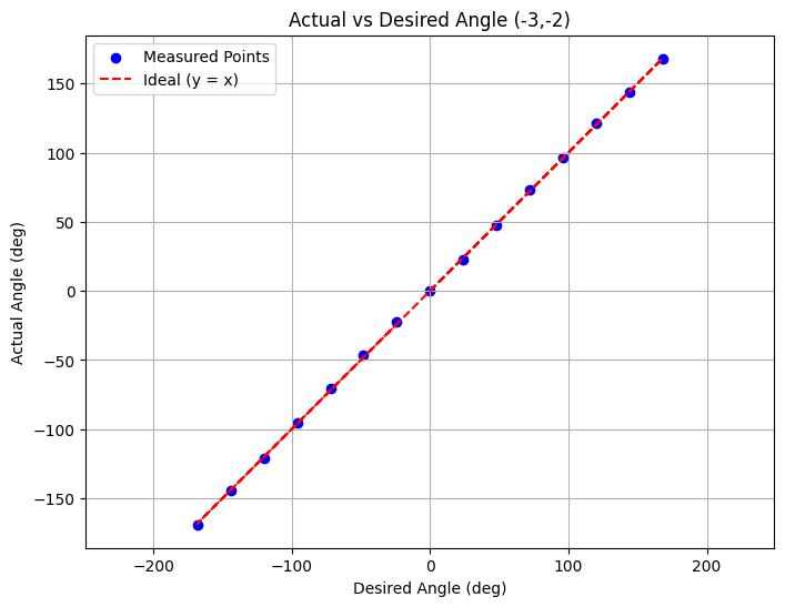
At each setpoint, I used a time-based approach to manage the PID iteration. The robot was given a 3-second window to stabilize and collect 10 distance measurements. In testing, this time frame consistently proved sufficient. I deliberately avoided techniques that rely on small PID outputs falling within the motor's deadband to bring the robot to a stop. Through experimentation, I found that as the battery voltage dropped, the effective deadband widened, leading to reduced angular accuracy. Instead, I allowed the PID controller to operate until the robot was within 2 degrees of the target angle before stopping. This method yielded reliable results, as demonstrated in the following plot of actual versus desired angles:
This 2-degree tolerance also informed my decision to record the DMP yaw angle alongside each distance measurement. By associating each distance reading with the actual yaw angle rather than the target setpoint, the precise angular accuracy relative to the setpoint became less critical. As long as enough measurements are taken throughout the rotation, mapping distances to the robot’s true orientation still allows for an accurate reconstruction of the environment.
In order to gain an understanding of the accuracy and precision I performed a rotation in the world at (-3,-2) I then took that data and took the mean and standard deviation of the 10 angle and distance measurements at each setpoint using this code:
angles = np.array(angle_strs, dtype=float)
distances = np.array(distance_strs, dtype=int)

angles_blocks = angles.reshape(-1, 10)
distances_blocks = distances.reshape(-1, 10)

angle_means = np.mean(angles_blocks, axis=1)
angle_stds = np.std(angles_blocks, axis=1)
distance_means = np.mean(distances_blocks, axis=1)
distance_stds = np.std(distances_blocks, axis=1)

for i in range(len(angle_means)):
    print(f"Angle {i+1}:")
    print(f"  Angle  → Mean: {angle_means[i]:7.3f}, Std Dev: {angle_stds[i]:6.3f}")
    print(f"  Distance → Mean: {distance_means[i]:7.1f}, Std Dev: {distance_stds[i]:6.1f}")
Angle 1:
  Angle  → Mean:  -0.001, Std Dev:  0.002
  Distance → Mean:   858.5, Std Dev:   18.8
Angle 2:
  Angle  → Mean:  22.625, Std Dev:  0.714
  Distance → Mean:   744.1, Std Dev:   19.8
Angle 3:
  Angle  → Mean:  47.712, Std Dev:  0.505
  Distance → Mean:   926.0, Std Dev:   62.0
Angle 4:
  Angle  → Mean:  71.464, Std Dev:  1.131
  Distance → Mean:   749.2, Std Dev:   47.4
Angle 5:
  Angle  → Mean:  96.612, Std Dev:  0.209
  Distance → Mean:   704.2, Std Dev:    1.5
Angle 6:
  Angle  → Mean: 119.440, Std Dev:  0.063
  Distance → Mean:   796.7, Std Dev:   17.6
Angle 7:
  Angle  → Mean: 145.480, Std Dev:  0.130
  Distance → Mean:   838.6, Std Dev:   23.9
Angle 8:
  Angle  → Mean: 169.046, Std Dev:  0.997
  Distance → Mean:   703.0, Std Dev:   11.5
Angle 9:
  Angle  → Mean: -169.267, Std Dev:  0.622
  Distance → Mean:   701.5, Std Dev:    5.4
Angle 10:
  Angle  → Mean: -143.615, Std Dev:  1.432
  Distance → Mean:   856.9, Std Dev:   30.0
Angle 11:
  Angle  → Mean: -120.060, Std Dev:  0.538
  Distance → Mean:   802.9, Std Dev:    7.9
Angle 12:
  Angle  → Mean: -96.902, Std Dev:  0.690
  Distance → Mean:   707.2, Std Dev:    4.2
Angle 13:
  Angle  → Mean: -72.254, Std Dev:  0.373
  Distance → Mean:  1002.0, Std Dev:  322.8
Angle 14:
  Angle  → Mean: -49.661, Std Dev:  1.511
  Distance → Mean:  1950.6, Std Dev:  308.3
Angle 15:
  Angle  → Mean: -25.945, Std Dev:  0.169
  Distance → Mean:  1666.9, Std Dev:   12.0
I then took the average of the mean and standard deviation across all 15 trials.
avg_angle_std = np.mean(angle_stds)
avg_distance_std = np.mean(distance_stds)

print(f"Average of angle std devs:     {avg_angle_std:.3f}°")
print(f"Average of distance std devs:  {avg_distance_std:.1f} mm")
Average of angle std devs:     0.606°
Average of distance std devs:  59.5 mm
The average of the angular standard deviations across all angles represents the typical noise level in the yaw measurements, providing an estimate of the consistency of the robot’s orientation data.
Similarly, the average of the distance standard deviations reflects the precision of the Time of Flight (ToF) sensor, indicating how tightly clustered the distance measurements are at each setpoint and thus serving as a measure of repeatability.
I then took 150 measurements at a range of 2m to gain an understanding of the accuracy.
mean_val = np.mean(values)
std_val = np.std(values)

print(f"Mean: {mean_val:.2f}")
print(f"Standard Deviation: {std_val:.2f}")
print(f"Mean Error: {2000-mean_val:.2f}")
Mean: 1934.42
Standard Deviation: 7.33
Mean Error: 65.58
import math

yaw_error_deg = 0.606
yaw_error_rad = math.radians(yaw_error_deg)

true_distance_mm = 2000
sensor_noise_mm = 59.5
sensor_bias_mm = 65.6

measured_distance_mm = true_distance_mm / math.cos(yaw_error_rad)
angular_error_mm = measured_distance_mm - true_distance_mm

total_rms_error = math.sqrt(
    angular_error_mm**2 +
    sensor_noise_mm**2 +
    sensor_bias_mm**2
)

worst_case_error = angular_error_mm + sensor_noise_mm + sensor_bias_mm

print(f"Angular error component: {angular_error_mm:.3f} mm")
print(f"Total RMS error: {total_rms_error:.2f} mm")
print(f"Worst case total error: {worst_case_error:.2f} mm")
Angular error component: 0.112 mm
Total RMS error: 88.56 mm
Worst case total error: 125.21 mm
This code estimates the effect of angular and sensor error on distance measurements. This is the case where the measured distance should be 2000 mm but we are assuming a yaw error of 0.606 degrees. The angular_error_mm is computed by comparing the measured distance, which is longer due to the angle error, to the true distance. Additionally, the found values for sensor noise and bias are included to calculate two overall error estimates: the root mean square (RMS) error, which combines all error sources in a way that accounts for the fact that not all the errors are correlated, and the worstcase error, which sums them directly to represent the maximum expected deviation. When measuring the closest point in the 4×4 m grid, we can expect an RMS error of 99.56 mm and a worst case error of 125.21 mm. I then repeated the same calculation for the farthest point in the grid, yielding an RMS error of 92.68 mm and a worst case error of 152.40 mm.
Read out Distances
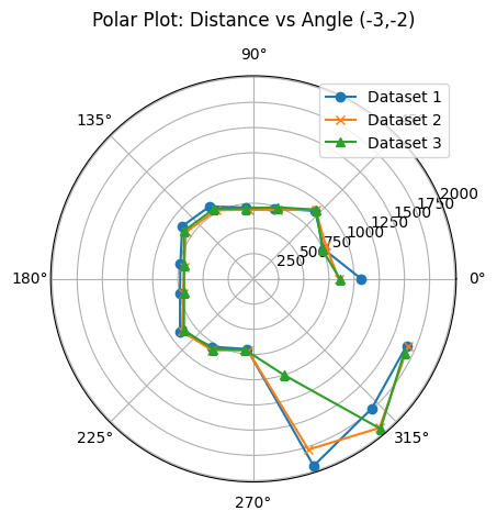
As a preliminary sanity check, I conducted three trials at the first measurement point (−3,−2). I overlaid the results on a single polar plot to verify consistency across trials. The corresponding polar plots were generated using the following code:
angles_rad = np.deg2rad(angles_deg)

plt.figure()
ax = plt.subplot(111, polar=True)
ax.plot(angles_rad, distances_mm, marker='o')
ax.set_title("Polar Plot: Distance vs Angle (-3,-2)", y=1.1)
plt.show()
Furthermore, after converting to cartesian coordinates, the plot output was consistent with the environment which can be observed below the polar plot.
(-3,-2)
.png)
(0,0)
.png)
.png)
(5,-3)
.png)
.png)
(0,3)
.png)
.png)
(5,3)
.png)
.png)
The conversion from polar to cartesian is performed using the matrices below which were discussed in lecture 2.
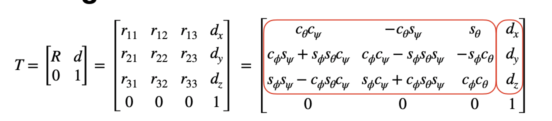
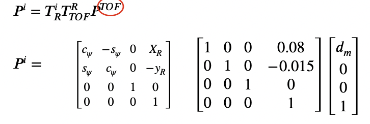
This was implemented in python using the following code which allowed me convert all my polar plots to cartesian plots.
x_R = -3 * 304.8
y_R = -2 * 304.8

x_global = []
y_global = []

for i in range(len(angles_rad)):
    theta = angles_rad[i]

    p_tof = np.array([[distances_mm[i]], [0], [0], [1]])

    T_tof_to_robot = np.array([
        [1, 0, 0, 0],
        [0, 1, 0, 0],
        [0, 0, 1, 0],
        [0, 0, 0, 1]
    ])

    cos_t = math.cos(-theta)
    sin_t = math.sin(-theta)
    T_robot_to_world = np.array([
        [cos_t, -sin_t, 0, x_R],
        [sin_t,  cos_t, 0, y_R],
        [0,      0,     1, 0],
        [0,      0,     0, 1]
    ])

    p_world = T_robot_to_world @ T_tof_to_robot @ p_tof

    x_global.append(p_world[0, 0])
    y_global.append(p_world[1, 0])

# Plotting
plt.figure(figsize=(6,6))
plt.plot(x_global, y_global, 'o')  # No connecting lines
plt.axis('equal')
plt.xlabel('X (mm)')
plt.ylabel('Y (mm)')
plt.title('Global Plot')
plt.grid(True)
plt.show()
After generating all of my cartesian plots I combined them all together to create a complete 2D map of the environment set up in the lab.
plt.figure(figsize=(8, 8))

plt.plot(x_global, y_global, 'o', label='Set 1')
plt.plot(x_global_2, y_global_2, 'o', label='Set 2')
plt.plot(x_global_3, y_global_3, 'o', label='Set 3')
plt.plot(x_global_4, y_global_4, 'o', label='Set 4')
plt.plot(x_global_5, y_global_5, 'o', label='Set 5')

plt.axis('equal')
plt.xlabel('X (mm)')
plt.ylabel('Y (mm)')
plt.title('All Global Plots')
plt.legend()
plt.grid(True)
plt.show()
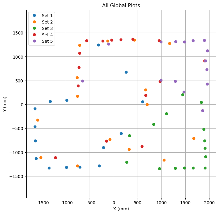
Surprisingly, the data closely resembled the actual environment. By following the general trends in the measurements, I was able to add boundaries that aligned well with the physical space.

Refrences
In Lab 9, I referenced Daria Kot's and Annabel Lian's webpages for guidance on generating Cartesian plots. I also used ChatGPT to assist with plot generation, Arduino debugging, and text editing. Additionally, it supported my analysis of accuracy and precision in the sensor data.